Comparative Analysis of Classification Algorithms
Comparative Analysis of Classification Algorithms
Abstract
This report provides a comprehensive analysis of the performance of three popular classification algorithms:
Decision Tree, Logistic Regression, Naive Bayes, Random Forest, Support Vector Machines (SVM) and Multilayer Perceptron.
The purpose of the study is to evaluate and compare these algorithms based on key performance metrics such as accuracy, precision, recall, F1-score, and false alarm rate (www.evidentlyai.com, n.d.), using two different datasets.
The dataset underwent preprocessing steps, including applying multiple scalers, normalization and handling of missing values, to ensure consistency and reliability of the results. The algorithms were trained and tested, with additional validation.
Confusion matrices (www.evidentlyai.com, n.d.) were used to visualize classification errors, while performance metrics were calculated for a detailed assessment.
- Random Forest consistently outperformed the other algorithms, achieving the highest accuracy of 95.2% and balanced metrics across classes.
- SVM demonstrated competitive performance but struggled with classes having overlapping distributions. Naive Bayes, while computationally efficient, showed limitations due to its independence assumption, resulting in lower precision for certain classes.
The results are presented through comparative tables and visualizations, providing actionable insights into the strengths and weaknesses of each algorithm. This analysis serves as a practical guide for selecting classification algorithms based on dataset characteristics and application requirements.
Introduction
The objective of this study is to compare various classification algorithms to evaluate their performance across key metrics, such as accuracy, precision, recall, and F1-score.
Classification plays a pivotal role in machine learning, enabling systems to categorize data effectively for decision-making tasks.
The algorithms explored include Decision Tree, Logistic Regression, Naïve Bayes, Random Forest, SVM-SVC, and MLP. The datasets are “NSL-KDD” AND “Processed Combined IoT dataset”. Preprocessing steps included handling missing values, scaling features, and encoding categorical data, preparing the dataset for optimal model performance.
Dataset Introduction
NSL-KDD
According to Gao(2019), the NSL-KDD dataset is a refined version of the original KDD’99 dataset, designed for evaluating intrusion detection systems (IDS). It addresses issues like redundant records and class imbalance, providing a balanced and reliable dataset. It includes 41 features per record and categorizes attacks into four types: DoS, Probe, R2L, and U2R. The dataset is divided into training and testing sets, with the testing set containing unseen attack types to evaluate generalization. Widely used for IDS research, feature engineering, and algorithm evaluation, NSL-KDD remains a popular benchmark, though its lack of modern threats highlights the need for complementary dataset.
Processed Combined IoT dataset
According to Alsaedi et al., the TON_IoT dataset is a new data-driven IoT/IIoT dataset. It includes heterogeneous data sources gathered from the Telemetry data of IoT/IIoT services, as well as the Operating Systems logs and Network traffic of IoT network, collected from a realistic representation of a medium-scale network. The dataset has various normal and attack events for different IoT/IIoT services, and includes a combination of physical and simulated IoT/IIoT services . The TON_IoT dataset aims to address the limitations of existing datasets by providing a more representative dataset for evaluating cybersecurity solutions and machine learning methods for IoT/IIoT applications . The dataset can be accessed through the TON-IoT repository.
Algorithms Overview
Decision Tree
Working Principle
A Decision Tree (scikit-learn, 2019) is a supervised learning algorithm used for both classification and regression tasks. It recursively splits the dataset into subsets based on feature values, creating a tree-like structure. Each internal node represents a decision based on a feature, while each leaf node represents the final predicted class or value. The tree construction process uses algorithms like ID3, CART, or C4.5, with the primary goal of reducing impurity at each split. Impurity is measured using metrics such as Gini Impurity or Entropy (for classification). The tree grows by selecting the feature that best separates the data at each node. Decision Trees are easy to understand and interpret, but they tend to overfit if not properly regularized.
Key Parameters
- max_depth: Limits the depth of the tree to avoid overfitting. A smaller depth prevents the model from capturing too much noise from the training data.
- min_samples_split: Specifies the minimum number of samples required to split an internal node. Larger values prevent the tree from becoming too specific to the training data.
- max_features: Defines the number of features to consider when looking for the best split. Reducing this value can speed up the training process and introduce diversity in ensemble methods like Random Forest.
- criterion: The function used to measure the quality of a split. It can be gini for Gini impurity or entropy for information gain.
Logistic Regression
Working Principle
Logistic Regression (scikit-learn, 2014) is a statistical method used for binary classification tasks. It predicts the probability that a given input belongs to a particular class. Unlike linear regression, which predicts continuous values, logistic regression applies a logistic (sigmoid) function to the output of a linear equation to map predictions to a probability between 0 and 1. The model learns by adjusting weights assigned to each feature to minimize the difference between predicted probabilities and actual class labels. Logistic Regression assumes a linear relationship between input features and the log odds of the target variable, making it simple yet effective for many classification problems.
Logistic Regression is widely used due to its simplicity, interpretability, and effectiveness in problems where the classes are linearly separable.
Key Parameters
- C: The regularization strength. It controls the trade-off between fitting the data well and preventing overfitting. Smaller values of C apply stronger regularization (higher penalty on complexity).
- solver: The algorithm used to optimize the weights of the model. Common solvers include liblinear, newton-cg, lbfgs, and saga. The solver choice affects convergence speed and suitability for certain datasets.
- max_iter: The maximum number of iterations for optimization algorithms. A higher value allows the algorithm to converge more precisely, especially for complex datasets.
- penalty: The regularization technique used. Common penalties include l2 (Ridge regularization), which discourages large coefficients, and l1 (Lasso), which encourages sparsity in the model.
- multi_class: Defines how multi-class classification is handled. Options include ovr (one-vs-rest) and multinomial. The choice depends on the problem being solved.
Naive Bayes
Working Principle
Naive Bayes (scikit-learn, n.d.) is a probabilistic algorithm based on Bayes’ Theorem, which calculates the posterior probability of a class given the features. It assumes independence among predictors, simplifying computations and making it efficient for high-dimensional data. Despite the naive assumption, it performs well in applications such as text classification and spam filtering. Naive Bayes is fast and computationally efficient, particularly for large datasets with independent features.
Key Parameters
- var_smoothing: A small additive constant to stabilize calculations and avoid division by zero when features have zero variance. Adjusting this parameter can help handle datasets with highly varying feature distributions.
Random Forest
Working Principle
Random Forest (scikit-learn, 2018) is an ensemble learning method that builds multiple decision trees during training and combines their predictions to improve classification accuracy and control overfitting. Each tree is trained on a bootstrap sample of the data, and feature selection at each node ensures diversity among the trees. For classification, the output is determined by majority voting among the trees. This method excels at handling large datasets with high dimensionality and is robust against noisy data.
Random Forest balances bias and variance effectively, making it suitable for diverse datasets.
Key Parameters
- n_estimators: The number of trees in the forest. Increasing this value improves accuracy but can increase computational cost.
- max_depth: The maximum depth of each tree. Limiting depth prevents overfitting while maintaining performance.
- min_samples_split: The minimum number of samples required to split a node. Higher values lead to simpler trees that generalize better.
Support Vector Machines (SVM)
Working Principle
SVM (scikit-learn, 2019) identifies a hyperplane that separates classes with the maximum margin. It uses kernel functions to transform data into higher dimensions for non-linear separation. By maximizing the margin, SVM minimizes classification error. It is effective for both linear and non-linear problems and is robust to overfitting, especially in highdimensional spaces.
SVM is versatile and powerful, particularly for datasets with complex decision boundaries.
Key Parameters
- c: The regularization parameter that controls the trade-off between achieving a low error on the training set and maintaining a large margin.
- kernel: Specifies the type of kernel function (e.g., linear, radial basis function (RBF), or polynomial). The choice depends on the dataset’s nature.
- gamma: The kernel coefficient for RBF and polynomial kernels, influencing the decision boundary’s flexibility. Lower values result in smoother boundaries, while higher values allow more complex boundaries.
Multilayer Perceptron
Working Principle
A Multilayer Perceptron (MLP) (scikit-learn, 2010) is a type of artificial neural network (ANN) composed of multiple layers of nodes (neurons). It consists of an input layer, one or more hidden layers, and an output layer. MLP is used for supervised learning tasks, such as classification and regression. The network learns by adjusting weights based on the errors between predicted and actual outputs using an optimization algorithm, typically backpropagation.
In MLP, the input data is passed through each layer of neurons. Each neuron applies a weighted sum of inputs, followed by an activation function to introduce non-linearity into the model. Common activation functions include ReLU (Rectified Linear Unit) for hidden layers and softmax for the output layer in classification tasks. During training, the model uses the backpropagation algorithm to compute the gradient of the loss function and update the weights accordingly. The goal is to minimize the difference between the predicted and actual output (i.e., minimize the loss).
MLP is a powerful model capable of learning complex patterns, making it well-suited for tasks such as image recognition, speech processing, and classification tasks that involve nonlinear decision boundaries. MLPs are versatile and can handle both simple and complex datasets. By adjusting the key parameters, MLPs can be fine-tuned for a variety of applications, including image recognition, natural language processing, and more.
Key Parameters
- hidden_layer_sizes: Defines the number and size of hidden layers in the network. For example, (100,) specifies a network with one hidden layer containing 100 neurons. The configuration of hidden layers affects the network**s ability to capture complex relationships.
- activation: Specifies the activation function used in the hidden layers. Common options include:
- relu: Rectified Linear Unit, a popular activation function that helps with faster training.
- tanh: Hyperbolic tangent, which outputs values between -1 and 1.
- logistic: Sigmoid function, often used for binary classification tasks.
- solver: The algorithm used for weight optimization. The common solvers are:
- adam: A popular optimization algorithm that adapts the learning rate during training.
- sgd: Stochastic Gradient Descent, a basic optimizer that updates weights based on a random subset of data.
- lbfgs: A quasi-Newton method, effective for smaller datasets.
- learning_rate: Determines how the learning rate changes during training. Options include:
- constant: The learning rate remains constant throughout training.
- invscaling: Gradually decreases the learning rate as training progresses.
- adaptive: The learning rate decreases when the validation score is not improving.
- max_iter: The maximum number of iterations for optimization. More iterations generally allow for better convergence, especially on more complex datasets.
- alpha: L2 regularization term that helps prevent overfitting by penalizing large weights. Higher values of alpha make the model simpler by forcing smaller weights.
- batch_size: The number of samples processed before the model updates its weights. Larger batch sizes lead to more stable but slower updates, while smaller batch sizes can speed up training but result in noisier updates.
Evaluation Metrics
Accuracy
The accuracy indicates the proportion of samples correctly classified by the model to the total number of samples.
Among them, $TP_i$ are the true positive examples of class i , and $FP_i$ are the false positive examples predicted as class i from other categories.
Precision
Precision is the proportion of correctly positive samples among all the samples predicted as positive. For each category i , the calculation formula for precision is:
Among them, $TP_i$ are the true positive examples of class i , and $FP_i$ are the false positive examples predicted as class i from other categories.
Recall
Recall is the proportion of correctly predicted positive samples among all the actual positive samples. For each category i , the calculation formula for precision is:
Among them, $TP_i$ are the true positive examples of class i , and $FN_i$ are the false positive examples predicted as class i from other categories.
F-Score
The F-Score is the harmonic mean of precision and recall. The calculation formula is:
False Alarm
FPR (False Positive Rate) is the proportion of negative samples that are incorrectly classified as positive among all actual negative samples. For each category i , the calculation formula for the false positive rate is:
Among them, $FP_i$ are the false positive examples predicted as class i from other categories, and $FP_i$ are the false positive examples predicted as class i from other categories.
Results and Analysis
Performance Metrics
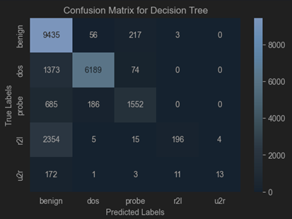
Decision Tree
According to the API documentation on scikit-learn, parameters such as max_depth, min_samples_split, min_samples_leaf, and criterion were tuned. The optimal parameter values were found to be: max_depth (default), min_samples_split=14, min_samples_leaf=2, and criterion=’gini’.
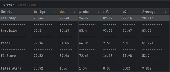
Dataset 1 (NSL-KDD)
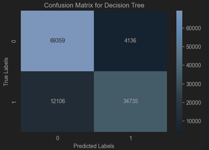
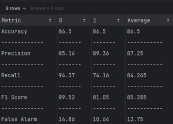
Dataset 2 (TON_IOT)
Comparing
| Metric | NSL-KDD (DT) | TON-IoT (DT) |
|---|---|---|
| Accuracy (%) | 90.846 | 86.5 |
| Precision (%) | 83.33 | 87.25 |
| Recall (%) | 51.274 | 84.265 |
| F-Score (%) | 53.2 | 85.285 |
| False Alarm (%) | 16.67 | 12.75 |
we can infer that the TON-IoT dataset generally yields better overall performance with the Decision Tree algorithm due to higher precision, recall, F-Score, and lower false alarm rates. In contrast, the NSL-KDD dataset achieves higher accuracy but struggles with recall and false alarm rates, possibly due to class imbalances or complexity in its features.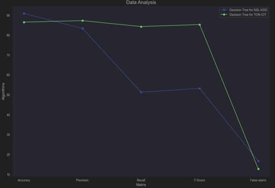
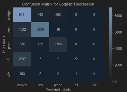
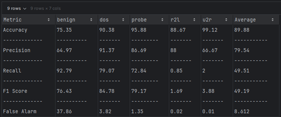
Logistic Regression
Logistic Regression provides several parameters that can be adjusted to change the behaviour of the model: Best parameters: {‘C’: 0.1, ‘penalty’: ‘l2’, ‘solver’: ‘lbfgs’}
Dataset 1 (NSL-KDD)
Dataset 2 (TON_IOT)
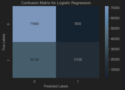
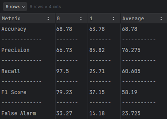
Comparing
| Metric | NSL-KDD (DT) | TON-IoT (DT) |
|---|---|---|
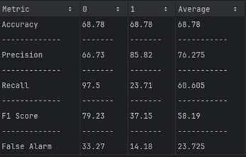
| Accuracy (%) | 89.88 | 68.78 |
| Precision (%) | 79.54 | 76.275 |
| Recall (%) | 49.51 | 60.605 |
| F-Score (%) | 49.19 | 58.19 |
| False Alarm (%) | 20.46 | 23.725 |
NSL-KDD Dataset: Logistic Regression is better at achieving higher accuracy and precision, making it more reliable for applications prioritizing these metrics.
TON-IoT Dataset: Logistic Regression is more effective at identifying true positives, as evidenced by its higher recall and F-Score, but it suffers from lower overall accuracy.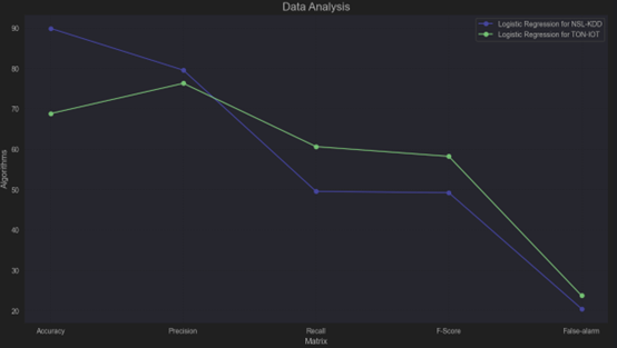
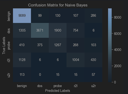
Naïve Bayes
From scikit-learn, we know that the performance of GaussianNB is depend on priors and var_smoothing. Best Parameters: {‘var_smoothing’: 1e-05}
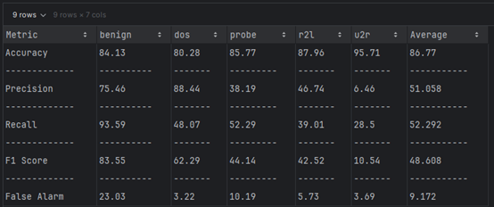
Dataset 1 (NSL-KDD)
Dataset 2 (TON_IOT)

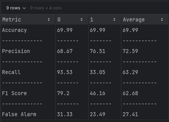
Comparing
| Metric | NSL-KDD (DT) | TON-IoT (DT) |
|---|---|---|
| Accuracy (%) | 86.77 | 69.99 |
| Precision (%) | 51.058 | 72.59 |
| Recall (%) | 52.292 | 63.29 |
| F-Score (%) | 48.608 | 62.68 |
| False Alarm (%) | 48.942 | 27.41 |
NSL-KDD Dataset: Naïve Bayes achieves high accuracy but struggles with false positives and balanced performance (F-Score).
TON-IoT Dataset: Naïve Bayes provides a more balanced classification with fewer false positives, making it better suited for use cases where precision and recall are critical.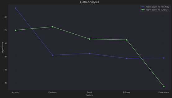
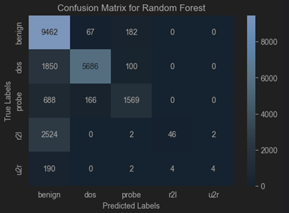
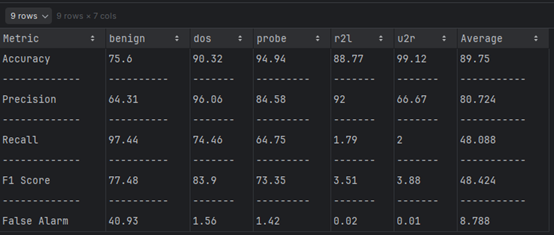
Random Forest
Random Forest has several important hyperparameters that we can adjust to improve its performance:
Best parameters found: {‘bootstrap’: False, ‘max_depth’: None, ‘min_samples_leaf’: 1, ‘min_samples_split’: 4, ‘n_estimators’: 33}
Dataset 1 (NSL-KDD)
Dataset 2 (TON_IOT)
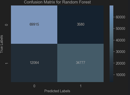
Comparing
| Metric | NSL-KDD (DT) | TON-IoT (DT) |
|---|---|---|
| Accuracy (%) | 89.75 | 86.96 |
| Precision (%) | 80.72 | 87.935 |
| Recall (%) | 48.088 | 84.64 |
| F-Score (%) | 48.424 | 85.745 |
| False Alarm (%) | 19.276 | 12.065 |
NSL-KDD Dataset: Random Forest achieves high accuracy but is less effective at achieving balanced precision and recall, with a moderate false alarm rate.
TON-IoT Dataset: Random Forest excels in all metrics, providing robust and balanced performance with minimal false alarms, making it a better-suited dataset for this algorithm.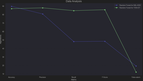
SVM-SVC
SVM-SVC has two important hyperparameters that we can adjust to improve its performance:
Best parameters: {‘C’: 1, ‘gamma’: ‘scale’}
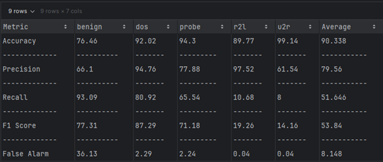
Dataset 1 (NSL-KDD)
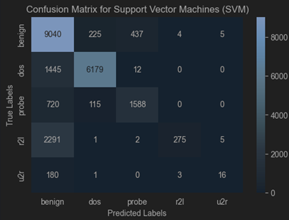
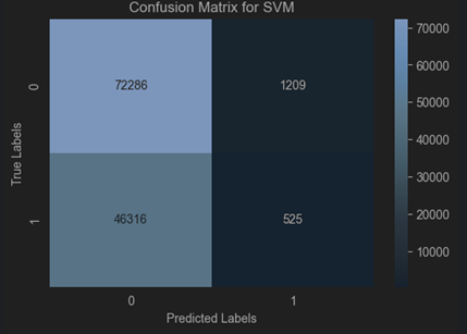
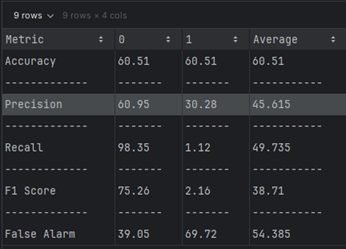
Dataset 2 (TON_IOT)
Best params: {‘kernel’: [‘poly’], ‘C’: [1 10*i for i in range(-3, 11)], ‘degree’: range(2, 10), ‘class_weight’: [‘balanced’], ‘max_iter’: [1000]}
Comparing
| Metric | NSL-KDD (DT) | TON-IoT (DT) |
|---|---|---|
| Accuracy (%) | 90.338 | 60.51 |
| Precision (%) | 79.56 | 45.615 |
| Recall (%) | 51.646 | 49.735 |
| F-Score (%) | 53.84 | 38.71 |
| False Alarm (%) | 20.44 | 54.385 |
NSL-KDD Dataset: SVM-SVC achieves excellent accuracy and precision but struggles with recall and balanced classification.
TON-IoT Dataset: SVM-SVC underperforms significantly, with low accuracy, precision, and F-Score, and a very high false alarm rate, suggesting it is not well-suited for this dataset without further tuning or preprocessing.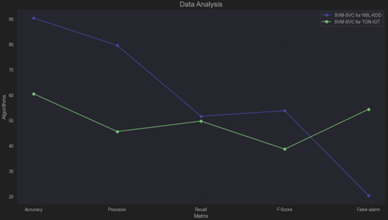
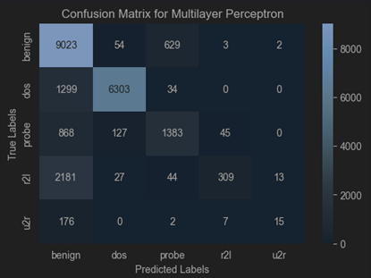
MLP
MLP has four important hyperparameters that we can adjust to improve its performance:
Best Parameters: {‘alpha’: 0.001, ‘hidden_layer_sizes’: (100,), ‘learning_rate_init’: 0.001, ‘solver’: ‘adam’}
Dataset 1 (NSL-KDD)
Dataset 2 (TON_IOT)
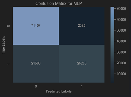
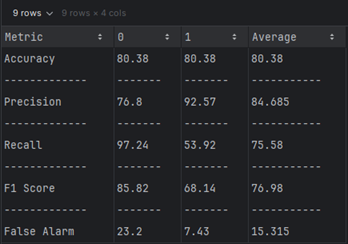
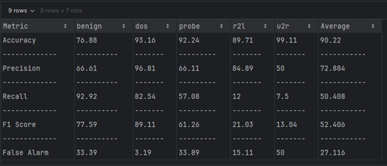
Comparing
| Metric | NSL-KDD (DT) | TON-IoT (DT) |
|---|---|---|
| Accuracy (%) | 90.22 | 80.38 |
| Precision (%) | 72.884 | 84.685 |
| Recall (%) | 50.408 | 75.58 |
| F-Score (%) | 52.406 | 76.98 |
| False Alarm (%) | 27.116 | 15.315 |
NSL-KDD Dataset: MLP achieves high accuracy but struggles with recall and false alarms, suggesting potential improvements through feature engineering or class balancing.
TON-IoT Dataset: MLP delivers robust performance with high precision, recall, and low false alarm rate, making it a strong candidate for this dataset.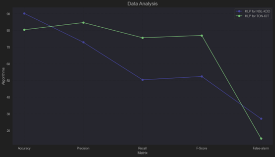
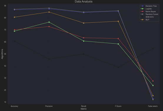
Summary
Dataset 1 (NSL-KDD)
| Algorithms | Accuracy (%) | Precision (%) | Recall (%) | F-Score (%) | False Alarm-FPR (%) | Times (s) |
|---|---|---|---|---|---|---|
| DeciTree | 90.846 | 83.33 | 51.274 | 53.2 | 16.67 | 1 |
| LR | 89.88 | 79.54 | 49.51 | 49.19 | 20.46 | 60 |
| NB | 86.77 | 51.058 | 52.292 | 48.608 | 48.942 | 15 |
| RanForest | 89.75 | 80.72 | 48.088 | 48.424 | 19.276 | 220 |
| SVM-SVC | 90.338 | 79.56 | 51.646 | 53.84 | 20.44 | 582 |
| MLP | 90.22 | 72.884 | 50.408 | 52.406 | 27.116 | 3600 |
Disscussion
In this analysis, we evaluate the performance of six classification algorithms—Decision Tree, Logistic Regression (LR), Naïve Bayes (NB), Random Forest (RF), SVM-SVC, and Multilayer Perceptron (MLP). The metrics considered include Accuracy, Precision, Recall, F1-Score, False Positive Rate (FPR), and execution time. Below is a summary of trends, dataset impact, and algorithm suitability based on the given dataset.
Performance Trends
- Accuracy
- Highest Accuracy: From Picture 25, we can see that Decision Tree (90.846%) and SVM-SVC (90.338%) are the best-performing algorithms.
- Lower Accuracy: Naive Bayes (86.77%), indicating it is less reliable for overall prediction correctness.
- Precision
- From the Picture 25, Decision Tree (83.33%), showing it has the fewest False Positives among all algorithms.
- Naïve Bayes showed the weakest precision (51.058%), aligning with its limited performance in complex datasets.
- Recall
- Naive Bayes (52.292%) and SVM-SVC (51.646%) perform best in detecting true positives.
- Random Forest (48.088%), indicating it misses many true positives.
- F1-Score
- SVM-SVC (53.84%) and Decision Tree (53.2%) provide the most balanced trade-off.
- Naive Bayes (48.608%) again struggles with performance consistency.
- False Positive Rate (FPR)
- Decision Tree (16.67%), making it the most reliable in minimizing False Alarms.
- Multi-Layer Perceptron (27.116%), which is prone to generating more False Alarms.
Impact of Dataset Characteristics
Decision Tree (DeciTree)
Strengths:- Accuracy (90.846%) and Precision (83.33%): Decision trees perform well for problems with simple decision boundaries, leading to good overall results. - Execution time (1 seconds): The algorithm is straightforward and efficient, making it suitable for small-scale datasets or simple problems.Weaknesses:
 - Low Recall (51.27%) and F1-Score (53.2%): Overfitting might result in poor recall for minority classes.
 - Susceptible to overfitting: When the dataset has noise or high-dimensional features, the model may capture irrelevant details, reducing generalization performance.
Logistic Regression (LR)
Strengths:- Balanced performance: As a linear model, LR works well for linearly separable data, achieving high precision 89.88%). - Efficient runtime (60 seconds): The algorithm is computationally efficient.Weaknesses:
 - Low Recall (49.51%) and F1-Score (49.19%): LR struggles with capturing complex nonlinear relationships, leading to lower recall and overall classification performance.
 - Dependency on feature relationships: LR assumes a linear relationship between features and outcomes, limiting its effectiveness on nonlinear datasets.
Naïve Bayes (NB)
Strengths:- Efficient computation: When the independence assumption holds, NB can quickly calculate posterior probabilities, making it suitable for tasks like text classification.Weaknesses:
- Low Accuracy (86.77%) and Precision (51.058%): The model struggles to utilize feature correlations effectively, as the independence assumption often doesn't hold, reducing its performance. - Low Recall (52.292%) and F1-Score (48.608%): Feature interdependence limits the model's effectiveness on complex datasets.- Random Forest (RanForest)
Strengths:
Weaknesses:- High Precision (89.75%): By aggregating multiple decision trees, Random Forest mitigates the overfitting issues of single trees. - Versatility: It can handle high-dimensional data and capture complex relationships.- High runtime (220 seconds): The complexity of the model significantly increases training and inference time compared to simpler algorithms. - Low Recall (48.088%) and F1-Score (48.424%): The model may not handle class imbalance well, requiring parameter tuning (e.g., class weights) to improve recall. - SVM-SVC
Strengths:
Weaknesses:- Adaptability to high-dimensional data: SVM with RBF kernels handles complex, nonlinear decision boundaries effectively. - Balanced performance: Accuracy (90.338%) and runtime (582 seconds) are relatively moderate.- Low Precision and Recall (51.646%, 53.84%): The model’s performance may be impacted by the complexity of data features and relationships. - High time complexity: Training time increases significantly for larger datasets. - Multilayer Perceptron (MLP)
Strengths:
Weaknesses:- Relatively stable Accuracy (90.22%) and F1-Score (52.406%): MLP effectively handles complex nonlinear problems. - Strong fitting ability: Particularly suitable for large-scale data with complex features.- High runtime (3600 seconds): Training neural networks is computationally expensive, especially for high-dimensional datasets. - Low Recall (50.408%): The model may not fully capture minority class characteristics due to insufficient parameter tuning or training data.
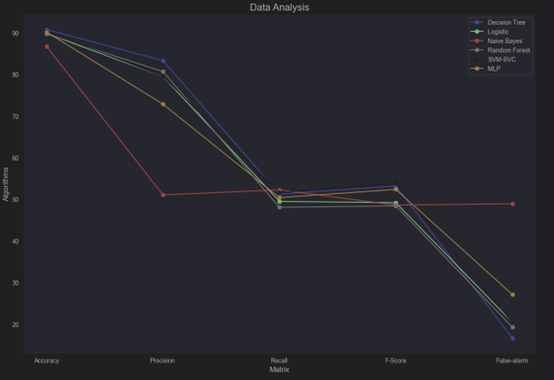
Dataset 2 (TON_IOT)
| Algorithms | Accuracy (%) | Precision (%) | Recall (%) | F-Score (%) | False Alarm-FPR (%) | Times (s) |
|---|---|---|---|---|---|---|
| DeciTree | 86.5 | 87.25 | 84.265 | 85.285 | 12.75 | 1 |
| LR | 68.78 | 76.275 | 60.605 | 58.19 | 23.725 | 319 |
| NB | 69.99 | 72.59 | 63.29 | 62.68 | 27.41 | 1 |
| RanForest | 86.96 | 87.935 | 84.64 | 85.745 | 12.065 | 43 |
| SVM-SVC | 60.51 | 45.615 | 49.735 | 38.71 | 54.385 | 3600 |
| MLP | 80.38 | 84.685 | 75.58 | 76.98 | 15.315 | 2115 |
Performance Trends
- Accuracy
- Best: Random Forest (86.96%) and Decision Tree (86.5%) are the most accurate.
- Worst: SVM-SVC (60.51%) has the lowest accuracy.
- Precision
- Best: Random Forest (87.935%) and Decision Tree (87.25%) again perform best in terms of precision.
- Worst: SVM-SVC (45.615%) significantly underperforms.
- Recall
- Best: Random Forest (84.64%) and Decision Tree (84.265%) lead in recall.
- Worst: SVM-SVC (49.735%).
- F-Score
- Best: Random Forest (85.745%) slightly edges out Decision Tree (85.285%).
- Worst: SVM-SVC (38.71%).
- False Alarm (FPR)
- Best: Random Forest (12.065%) and Decision Tree (12.75%) maintain low false positive rates.
- Worst: SVM-SVC (54.385%) is the highest.
- Execution Time
- Fastest: Decision Tree (1 second) and Naïve Bayes (1 second).
- Slowest: SVM-SVC (3600 seconds), followed by MLP (2115 seconds).
Impact of Dataset Characteristics
Dimensionality:
TON_IoT likely involves high-dimensional data due to its IoT nature, affecting algorithm performance:
- Random Forest and Decision Tree, with their ability to handle high-dimensional datasets and irrelevant features, perform well.
- SVM-SVC, which struggles with large datasets, reflects this limitation in its performance.
Noise and Outliers:
IoT datasets often include noisy data:
- Random Forest and Decision Tree mitigate noise with feature averaging and robust splitting.
- MLP may struggle with noise, requiring substantial preprocessing for optimal results.
- Naïve Bayes, assuming feature independence, may be sensitive to outliers, though its simplicity helps in certain cases.
Class Imbalance:
IoT datasets often exhibit class imbalance (e.g., rare attack types vs. normal behavior). Algorithms handling imbalance:
- Random Forest and Decision Tree, using ensemble learning and weighted splits, manage imbalance better.
- Logistic Regression and Naïve Bayes may underperform in imbalanced scenarios without appropriate resampling techniques.
- SVM-SVC is particularly sensitive to imbalance, resulting in poor metrics.
Conclusion
In conclusion, the strengths and weaknesses of each algorithm are influenced by their underlying assumptions, model complexity, and adaptability to the dataset. For simple problems or scenarios requiring high efficiency, Decision Tree or Logistic Regression is recommended. Random Forest and MLP perform better on complex datasets but come with higher computational costs. SVM-SVC is well-suited for high-dimensional, nonlinear data, while Naïve Bayes can be effective for specific tasks such as text classification.
Reference
- Alsaedi, Abdullah, et al. “TON_IoT Telemetry Dataset: A New Generation Dataset of IoT and IIoT for Data-Driven Intrusion Detection Systems.” IEEE Access, 2020, pp. 1–1, https://doi.org/10.1109/access.2020.3022862.
- Gao, X., Shan, C., Hu, C., Niu, Z. and Liu, Z., 2019. An adaptive ensemble machine learning model for intrusion detection. Ieee Access, 7, pp.82512-82521.
- Scikit-learn.org. (2019). sklearn.tree.DecisionTreeClassifier — scikit-learn 0.22.1 documentation. [online] Available at: https://scikit-learn.org/stable/modules/generated/sklearn.tree.DecisionTreeClassifier.html.
- scikit-learn (2014). sklearn.linear_model.LogisticRegression — scikit-learn 0.21.2 documentation. [online] Scikit-learn.org. Available at: https://scikit-learn.org/stable/modules/generated/sklearn.linear_model.LogisticRegression.html.
- scikit-learn (n.d.). sklearn.naive_bayes.GaussianNB — scikit-learn 0.22.1 documentation. [online] scikit-learn.org. Available at: https://scikit-learn.org/stable/modules/generated/sklearn.naive_bayes.GaussianNB.html.
- Scikit-learn.org. (2018). sklearn.ensemble.RandomForestClassifier — scikit-learn 0.20.3 documentation. [online] Available at: https://scikit-learn.org/stable/modules/generated/sklearn.ensemble.RandomForestClassifier.html.
- scikit-learn (2019). sklearn.svm.SVC — scikit-learn 0.22 documentation. [online] Scikit-learn.org. Available at: https://scikit-learn.org/stable/modules/generated/sklearn.svm.SVC.html.
- scikit-learn (2010). sklearn.neural_network.MLPClassifier — scikit-learn 0.20.3 documentation. [online] Scikit-learn.org. Available at: https://scikit-learn.org/stable/modules/generated/sklearn.neural_network.MLPClassifier.html.
- SciKit Learn (2019). sklearn.model_selection.GridSearchCV — scikit-learn 0.22 Documentation. [online] Scikit-learn.org. Available at: https://scikit-learn.org/stable/modules/generated/sklearn.model_selection.GridSearchCV.html.
- www.evidentlyai.com. (n.d.). How to interpret a confusion matrix for a machine learning model. [online] Available at: https://www.evidentlyai.com/classification-metrics/confusion-matrix.
- www.evidentlyai.com. (n.d.). Accuracy vs. precision vs. recall in machine learning: what’s the difference? [online] Available at: https://www.evidentlyai.com/classification-metrics/accuracy-precision-recall#what-is-recall.