Machine Learning
Overview of Machine Learning
What is Machine Learning?
Machine Learning (ML) is a subset of artificial intelligence (AI) that enables computers to learn from data and improve their performance over time without being explicitly programmed. ML algorithms build mathematical models based on sample data, known as “training data,” to make predictions or decisions without being explicitly programmed to perform the task.
Artificial intelligence is a field of computer science that aims to create machines that can perform tasks that normally require human intelligence. Includes Natural Language Processing (NLP), Computer Vision, Robotics, and more.
Machine learning is a subset of AI that enables computers to learn from data and improve their performance over time without being explicitly programmed.
Deep learning is a subset of machine learning that uses neural networks with many layers to model complex patterns in data.
Key Concepts in Machine Learning
- Dataset: A collection of data used for training and testing ML models.
- Training Set: The portion of the dataset used to train the model.
- Testing Set: The portion of the dataset used to evaluate the model’s performance
- Validation Set: A separate subset of the dataset used to validate the model’s performance.
- Samples: Individual data points in the dataset.
- Features: The attributes or properties of the data that are used for making predictions.
- Feature Vectors: A representation of features in a numerical format that can be processed by ML algorithms.
- Labels: The target variable that the model is trying to predict (in supervised learning).
- Model: The mathematical representation learned from data, used to make predictions.
- Parameters: The internal variables of the model that are learned from the training data.
- Hyperparameters: Parameters that are not learned from the training data, but are set by the user.
Machine Learning Fundamental Theorem
Three Elements of Machine Learning
Machine learning relies on three fundamental elements:
- Model: Summarizes the inherent patterns in the data and describes the parameter system using mathematical language.
- Strategy: Evaluation criteria for selecting the optimal model.
- Algorithm: Specific methods for selecting the optimal model.
Types of Machine Learning
- Supervised Learning: The model learns from labeled data (e.g., classification, regression), where the model is provided with input-output pairs.
- Unsupervised Learning: The model finds patterns in unlabeled data (e.g., clustering, dimensionality reduction), where the model is provided with input data and must find hidden structures.
- Reinforcement Learning: The model learns by interacting with an environment and receiving feedback (rewards or penalties), where the model is provided with input-output pairs.
- Supervised Learning
- Linear Model
- Linear Regression
- Lasso Regression
- Ridge Regression
- Linear Discrimination Analysis (LDA)
- Logistic Regression
- K-Nearest Neighbors (KNN)
- Decision Trees
- Naive Bayes
- Support Vector Machines (SVM)
- Neural Networks
- Ensemble Learning
- Boosting
- AdaBoost
- Gradient Boosting trees
- XGBoost
- LightGBM
- Bagging
- Random Forest
- Boosting
- Linear Model
- Unsupervised Learning
- Clustering
- K-Means
- Gaussian Mixture Clustering
- Density Clustering
- Hierarchical Clustering
- Spectral Clustering
- Dimensionality Reduction
- Main Component Analysis (PCA)
- Singular Value Decomposition (SVD)
- t-SNE
- Self-encoder
- Clustering
- Semi-Supervised Learning
- Semi-Supervised Support Vector Machines (S3VM)
- Graph-Based Semi-Supervised Learning
- Generative Models
- Collaborative training
- Reinforcement Learning
- Dynamic Programming
- Monte Carlo Tree Search
- Q-Learning
- Strategic Gradient Algorithms
- Mimicking Learning
Probabilistic Model
- EM Algorithm
- Naive Bayes
- Bayesian Networks
- Hidden Markov Models
- Markov Random Fields
- Conditional Random Fields
- Markov Chain Monte Carlo
- Hidden Dirichlet Allocation (LDA)
- Variational Autoencoders (VAE)
Modeling Process
- Data Collection: Gathering data from various sources.
- Data Cleaning: Handling missing values, removing duplicates, and correcting errors in the data.
- Feature Engineering: Creating new features from existing data to improve model performance.
- Algorithm Selection: Choosing the appropriate machine learning algorithm based on the problem and data characteristics.
- Model Training: Training the selected algorithm on the prepared data.
- Model Evaluation: Assessing the performance of the trained model using appropriate metrics.
- Model Optimization: Tuning hyperparameters and improving the model based on evaluation results.
- Model Deployment: Deploying the trained model into a production environment for real-world use.
Feature Engineering
Feature engineering is the process of creating new features from existing data to improve the performance of machine learning models. It involves techniques such as:
- Feature Selection: Selecting the most relevant features for model training to reduce dimensionality and improve model performance.
- Filter Methods: The relationship between features and the target variable is evaluated based on statistical tests (e.g., chi-square test, correlation coefficient, information gain), and the most relevant features are selected.
- Wrapper Methods: Use models(such as Recursive Feature Elimination, RFE) to evaluate the importance of features and select features based on the model’s performance.
- Embedded methods: Use the model’s own feature selection mechanism (such as feature importance in decision trees, L1 regularized feature selection) to select the most important features.
- Feature Transformation: Applying mathematical operations to the features to normalize or scale them (e.g., logarithmic transformation for non-negative data).
- Normalization: Scales features to a specific range (typically between 0 and 1). Suitable for scale-sensitive models (such as KNN and SVM).
- Standardization: By subtracting the mean and dividing by the standard deviation, the distribution of the feature is made to have a mean of 0 and a standard deviation of 1. Suitable for scale-insensitive models (such as linear regression).
- Log Transformation: For skewed distributions (such as income, prices, etc.), logarithmic transformation can convert them into a form that is closer to a normal distribution.
- Encoding of categorical variables
- One-hot encoding: Converting categorical variables into binary columns is often used for unordered categorical features.
- Label encoding: Mapping categorical variables to integers is often used for ordinal categorical features.
- Target encoding: Replace each category of the categorical variable with the mean or other statistic of its corresponding target variable.
- Frequency encoding: Replace each category of the categorical variable with the frequency of that category in the dataset.
- Feature Construction: Feature construction involves creating new, more representative features based on existing features. By combining, transforming, or aggregating existing features, features that better reflect the patterns in the data can be formed.
- Interactive Feature: Combining two features to form a new feature. For example, the product, sum, or difference of two features. For example, combining age and income to create a new feature may better reflect certain patterns.
- Statistical Features: Extracting statistical values from original features, such as calculating the average, maximum, minimum, and standard deviation for a given time window. For example, in time series data, you can extract the average for each hour or day from the original data.
- Date and Time Features: Extracting features such as day of the week, month, year, and quarter from date and time data. For example, converting “2000-01-01” into features such as “day of the week,” “whether it’s a holiday,” and “beginning or end of the month.”
- Feature Dimensionality Reduction: When the number of features in a dataset is very large, feature dimensionality reduction can help reduce computational complexity and avoid overfitting. Dimensionality reduction methods can reduce the number of features while preserving the essence of the data.
- Principal Component Analysis (PCA): Maps the original features to a new space through linear transformation, so that the new features (principal components) retain the variance of the data as much as possible.
- Linear Discriminant Analysis (LDA): A supervised learning dimensionality reduction method that reduces dimensionality by maximizing the ratio of inter-class distance to intra-class distance.
- t-SNE (t-Distributed Stochastic Neighbor Embedding): A non-linear dimensionality reduction technique, particularly suitable for visualizing high-dimensional data.
- Autoencoder: A neural network model that achieves dimensionality reduction of data through a compression encoder.
Low Variance Filtering Method
Feature selection can be based directly on variance, which is the simplest approach. Features with low variance mean that all sample values for that feature are almost identical, having minimal impact on prediction, and can be removed.1
2
3
4
5
6
7
8
9
10
11
12
13
14from sklearn.feature_selection import VarianceThreshold
# Create a VarianceThreshold object
selector = VarianceThreshold(threshold=0.1)
selector.fit_transform(X)
# Get the feature ranking
ranking = selector.get_support(indices=True)
# Get the feature names
feature_names = selector.get_feature_names()
# Get the feature names and ranking
feature_names, ranking = selector.get_feature_names_out()
Correlation-Based Feature Selection
Correlation-based methods evaluate the relationship between features and the target variable, or among features themselves.
They are commonly used to:
- Select highly relevant features (strong correlation with the target)
- Remove redundant features (high correlation between features)
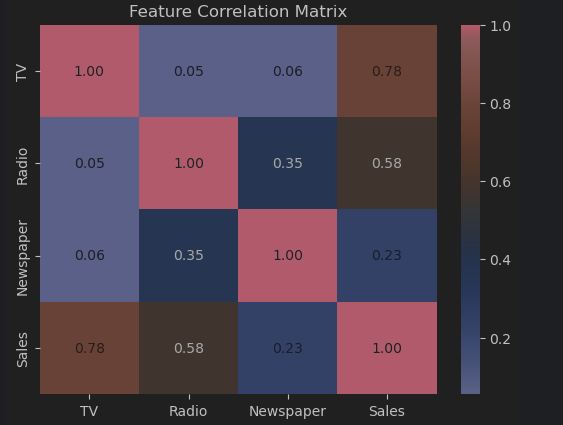
Pearson Correlation Coefficient
The Pearson Correlation Coefficient measures the linear relationship between two variables. Its value ranges from -1 to 1.
- Positive Correlation (r → 1): As the feature increases, the target variable also increases.
- Negative Correlation (r → -1): As the feature increases, the target variable decreases.
- No Correlation (r → 0): No clear relationship between the feature and the target variable.
Example
Suppose we have a dataset containing advertising spending across different channels and sales revenue.
We can compute the Pearson correlation coefficient between each feature and the target using:1
pandas.DataFrame.corrwith(method="pearson")
1 | import pandas as pd |
Spearman Rank Correlation Coefficient
The Spearman Rank Correlation Coefficient (Spearman’s ρ) is defined as the Pearson correlation coefficient between the ranked variables.
It measures the monotonic relationship between two variables — that is, whether one variable consistently increases or decreases as the other increases (not necessarily linearly).
- Suitable for non-linear relationships
- Does not require normal distribution
- Works well with ordinal (ranked) data
Where:
- $d_i$ = difference between the ranks of each pair of observations
- $n$ = number of samples
- ρ = 1: Perfect positive correlation (as one variable increases, the other always increases)
- ρ = -1: Perfect negative correlation (as one variable increases, the other always decreases)
- ρ = 0: No correlation
Example
Suppose we have a dataset of weekly study hours (X) and math exam scores (y):
| X (Hours) | y (Score) |
|---|---|
| 5 | 55 |
| 8 | 65 |
| 10 | 70 |
| 12 | 75 |
| 15 | 85 |
| 3 | 50 |
| 7 | 60 |
| 9 | 72 |
| 14 | 80 |
| 6 | 58 |
Step 1: Rank the Data
| X | Rank(X) | y | Rank(y) | d = RX - Ry | d² |
|---|---|---|---|---|---|
| 5 | 2 | 55 | 2 | 0 | 0 |
| 8 | 5 | 65 | 5 | 0 | 0 |
| 10 | 7 | 70 | 6 | 1 | 1 |
| 12 | 8 | 75 | 8 | 0 | 0 |
| 15 | 10 | 85 | 10 | 0 | 0 |
| 3 | 1 | 50 | 1 | 0 | 0 |
| 7 | 4 | 60 | 4 | 0 | 0 |
| 9 | 6 | 72 | 7 | -1 | 1 |
| 14 | 9 | 80 | 9 | 0 | 0 |
| 6 | 3 | 58 | 3 | 0 | 0 |
Step 2: Compute Spearman Correlation
1 | df.corrwith(target, method="spearman") |
1 | import pandas as pd |
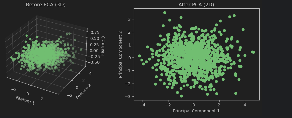
Principal Component Analysis (PCA)
Principal Component Analysis (PCA) is a statistical procedure that uses an orthogonal transformation to convert a set of observations of possibly correlated variables into a set of values of linearly uncorrelated variables called principal components.
Principal component analysis is performed using sklearn.decomposition.PCA. The parameter n_components, if a decimal, indicates the proportion of information to retain; if an integer, it indicates the number of dimensions to retain.
1 | import numpy as np |
Model Evaluation and Model Selection (Key Topic)
Loss Function
To evaluate how good a model’s prediction is, we need a measurement criterion.
In supervised learning, given an input $X$, a model can be viewed as a decision function $f$, which outputs a prediction $f(X)$.
The true label is denoted as $Y$.
There is usually a deviation between $f(X)$ and $Y$, which is measured by a loss function:
Properties of Loss Functions
- A loss function measures the prediction error of a model
- The smaller the loss value, the better the model
- The loss function is a non-negative real-valued function of $f(X)$ and $Y$
Common Loss Functions
1. 0-1 Loss Function
2. Squared Loss Function
3. Absolute Loss Function
4. Log-Likelihood Loss (Negative Log-Likelihood)
Empirical Error (Empirical Risk)
Given a training dataset with $n$ samples:
Using a chosen loss function, we can compute the average error on the training set, known as:
- Training Error
- Empirical Error
- Empirical Risk
Generalization Error
Similarly, the average error on the test dataset is called:
- Test Error
- Generalization Error
This reflects how well the model performs on unseen data.
Model Evaluation Strategy
A common evaluation strategy is to analyze the empirical error:
- When the empirical risk is minimized, the model is considered optimal under this criterion
- This principle is known as Empirical Risk Minimization (ERM)
Underfitting and Overfitting
Fitting refers to the process by which a machine learning model learns patterns from training data and makes predictions.
Ideally, a model should:
- Capture the underlying patterns in the training data
- Perform well on unseen data (test data)
This ability is known as generalization.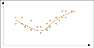
Underfitting occurs when a model performs poorly on the training data and fails to capture the underlying patterns.
- Poor performance on both training and test datasets
- Model is too simple
- Characterized by high bias
Overfitting occurs when a model performs very well on training data but poorly on unseen data.
- Very low error on training data
- High error on test data
- Model learns noise and details instead of general patterns
- Characterized by high variance
Root Cause
The fundamental cause of underfitting and overfitting is model complexity:
- Too simple → Underfitting
- Too complex → Overfitting
This leads to high generalization error.
Comparison
| Type | Training Error | Test Error | Model Complexity | Key Issue |
|---|---|---|---|---|
| Underfitting | High | High | Too simple | High Bias |
| Overfitting | Low | High | Too complex | High Variance |
Causes and Solutions
Underfitting
Causes:
Insufficient model complexity
The model is too simple to capture complex relationshipsInsufficient features
Poor feature selection or lack of informative featuresInsufficient training
Too few training iterationsExcessive regularization
Regularization is too strong, forcing the model to be overly simple
Solutions:
- Increase model complexity
- Add more features or improve feature engineering
- Train longer (more iterations)
- Reduce regularization strength
Overfitting
Causes:
Excessive model complexity
Too many parametersInsufficient training data
Model memorizes training data instead of learning patternsToo many features
Model captures noise instead of useful signalOvertraining
Training too long causes the model to fit noise
Solutions:
- Reduce model complexity (simpler models, dimensionality reduction)
- Increase training data (or use data augmentation)
- Apply regularization (L1, L2)
- Use cross-validation
- Apply early stopping (stop when validation loss stops improving)
Summary
- Underfitting: high bias, model too simple
- Overfitting: high variance, model too complex
- The goal is to find a balance that minimizes generalization error
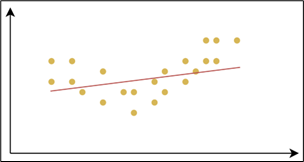
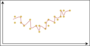
Example
Fit sin(x) to x∈[-3,3] using a polynomial:
1 | import numpy as np |
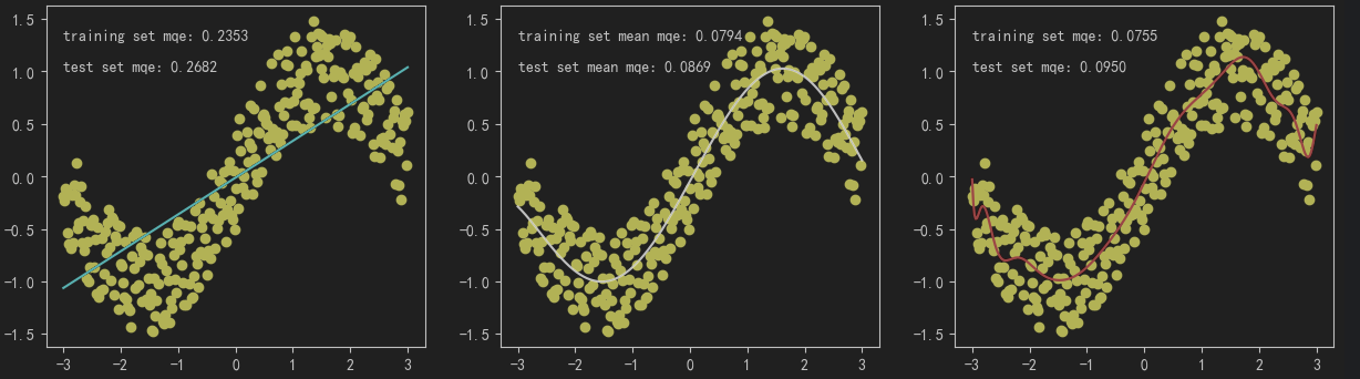
Conclusion:
When the polynomial degree is low, the model is too simple and the fit is poor.
As the polynomial degree increases, the model complexity becomes moderate, the fit is good, and both training and test errors are low.
When the polynomial degree continues to increase, the model becomes too complex, overlearns noise, resulting in low training error but high test error.
Regularization
Regularization is a technique used in machine learning to prevent overfitting by adding a penalty term to the loss function.
This penalty discourages overly large model parameters, thereby:
- Reducing model complexity
- Improving generalization performance
Regularized Loss Function
For example, adding a regularization term to the squared loss:
Original loss term:
→ Fits the training data
Regularization term:
→ Penalizes large parameters and reduces model complexity
Regularization Coefficient: $\lambda$ is the regularization coefficient, it controls the strength of the penalty and it is a hyperparameter (not learned during training).
Trade-off:
- Large $\lambda$ → simpler model → risk of underfitting
- Small $\lambda$ → complex model → risk of overfitting
L1 Regularization (Lasso)
Characteristics
- Encourages some weights to become exactly zero
- Performs feature selection automatically
- Produces a sparse model
In regression problems, this is known as Lasso Regression.
L2 Regularization (Ridge)
Characteristics
- Shrinks all weights toward zero, but not exactly zero
- Produces a smooth and stable model
- Helps reduce overfitting without eliminating features
In regression problems, this is known as Ridge Regression.
Elastic Net Regularization
Elastic Net combines both L1 and L2 regularization:
Parameters
- $\lambda$: overall regularization strength
- $\alpha \in [0,1]$: balance between L1 and L2
Characteristics
- Combines:
- Sparsity (from L1)
- Stability (from L2)
- Useful when:
- Features are highly correlated
- You want both feature selection and robustness
Summary
- Regularization reduces overfitting by penalizing large parameters
- L1 → sparse model (feature selection)
- L2 → smooth model (weight shrinkage)
- Elastic Net → balance between L1 and L2
- $\lambda$ controls the bias–variance tradeoff
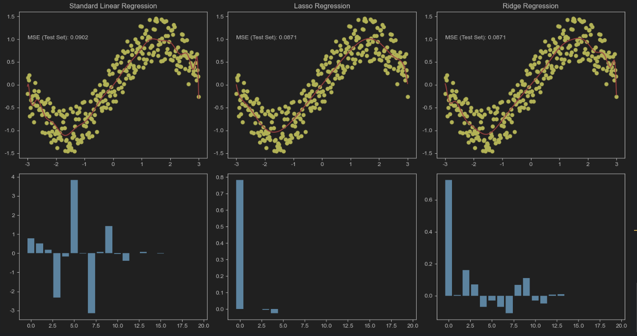
Example
Similarly, taking the example of fitting sin(x) on x∈[-3,3] using a polynomial, we will perform fitting without regularization, with L1 regularization, and with L2 regularization.
1 | import numpy as np |
Cross-Validation
Cross-Validation is a technique used to evaluate a model’s generalization ability.
It works by splitting the dataset into multiple subsets and repeatedly training and validating the model. This helps:
- Reduce randomness caused by a single data split
- Provide a more reliable estimate of performance on unseen data
- Mitigate risks of overfitting and underfitting due to poor data partitioning
Hold-Out Validation
The dataset is split into two parts:
- Training set (e.g., 70%)
- Validation set (e.g., 30%)
Characteristics
- Simple and fast
- Performance depends heavily on a single split
- May overestimate or underestimate model performance
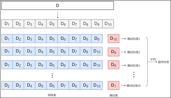
k-Fold Cross-Validation
The dataset is divided into $k$ equal subsets (called folds).
Procedure
- Split data into $k$ folds
- For each iteration:
- Use $k - 1$ folds for training
- Use the remaining 1 fold for validation
- Repeat $k$ times
- Compute the average performance
Characteristics
- Efficient use of data
- More stable and reliable results
- Widely used in practice
Leave-One-Out Cross-Validation (LOOCV)
A special case of k-fold where $k$ equals the number of samples. Each sample is used once as a validation set while the rest form the training set.
Summary
| Method | Data Usage | Stability | Computational Cost | Notes |
|---|---|---|---|---|
| Hold-Out | Low | Low | Low | Simple but unstable |
| k-Fold | High | High | Medium | Most commonly used |
| LOO | Very High | Very High | Very High | Best for small datasets |
Model Optimization Algorithms
Regularization helps prevent overfitting and improves generalization.
In this case, the model evaluation strategy becomes minimizing the regularized empirical risk, known as Structural Risk Minimization (SRM).
This is essentially an optimization problem, where the objective function depends on model parameters $\theta$.
Solution Methods
There are two main approaches to solving this optimization problem:
- Analytical Solution (Closed-form)
- Iterative Methods (e.g., Gradient Descent)
Analytical Solution
If the minimum of the loss function can be derived mathematically, we can directly compute the optimal parameters.
Characteristics
- Conditions: The function must be differentiable and solvable analytically
- Advantages: Exact and efficient
- Disadvantages: Limited applicability; expensive for high-dimensional data
Example: Linear Regression (Least Squares)
Linear regression problems: analytical solutions can be obtained using the “least squares method”.
Linear regression L2 regularization (Ridge regression)
The term $\lambda I$ stabilizes the matrix inversion, hence the name Ridge Regression.
Gradient Descent (Key Method)
Gradient Descent is a widely used first-order iterative optimization algorithm.
Core Idea
- Start with an initial parameter $\theta_0$
- Update parameters iteratively in the negative gradient direction
- Continue until convergence
Update Rule:
Where:
- $\nabla L(\theta_k)$ = gradient of the loss function
- $\alpha$ = learning rate (hyperparameter)
Key Concepts
- Gradient direction: fastest increase of the function
- Negative gradient: fastest decrease → used for minimization
Characteristics
- May converge to a local minimum (not always global)
- Advantages: simple, widely applicable
- Disadvantages: may be slow; sensitive to learning rate
Types of Gradient Descent
Batch Gradient Descent (BGD)
Uses the entire training dataset to compute the gradient at each iteration.
Pros: easy to implement; Stable convergence
Cons: requires the entire dataset; may be slow for large datasets, High computational cost per iteration
Stochastic Gradient Descent (SGD)
Uses one sample at a time to compute the gradient.
Pros: Fast; can be used for large datasets; can be used for small datasets
Cons: Noisy updates; unstable convergence; may require more iterations to converge
Mini-Batch Gradient Descent (MBGD)
Uses a small batch of samples to compute the gradient at each iteration.
Pros: Balance between BGD and SGD; faster convergence; more stable than SGD
Cons: requires a small batch size; may be slow for large datasets
Gradient Descent Procedure
- Initialize parameters randomly
- Compute gradient of the loss function
- Update parameters using gradient
- Repeat until stopping criteria:
- Gradient ≈ 0
- Max iterations reached
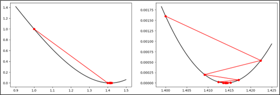
Example: Gradient Descent
Given:
Find $x$ such that $f(x) = 2$
Define objective function:
Gradient:
- Initial value: $x_1 = 1$
- Learning rate: $\alpha = 0.1$
Step 1:
Step 2:
Final convergence:
1 | def J(x): |
L1 Regularization (Lasso)
Gradient Derivation
Where:
Parameter Update Rule
The gradient of the L1 regularization term is a constant:
When $\omega_j$ is small, it can be driven directly to zero . This leads to sparsity → automatic feature selection
L2 Regularization (Ridge)
Loss Function
Gradient Derivation
Parameter Update Rule
Key Insight
- The gradient of the L2 term is proportional to $\omega_j$:
- Each update shrinks the parameter toward zero
- Parameters become small but not exactly zero
- Leads to a smooth and stable model
Comparison
| Aspect | L1 (Lasso) | L2 (Ridge) | ||
|---|---|---|---|---|
| Penalty | $ | \omega | $ | $\omega^2$ |
| Gradient | Constant | Proportional to $\omega$ | ||
| Sparsity | Yes (many zeros) | No | ||
| Feature Selection | Yes | No | ||
| Model Behavior | Sparse | Smooth |
- L1 → drives parameters to zero → feature selection
- L2 → shrinks parameters → stability & regularization
- Both reduce overfitting but behave differently during optimization
Newton’s Method and Quasi-Newton Methods (Overview)
Newton’s Method is a classical optimization technique for solving unconstrained optimization problems.
It uses second-order derivative information (the Hessian matrix) to iteratively approach the optimal solution.
Update Rule
Where:
- $\nabla L(\theta_k)$ = gradient of the loss function
- $H^{-1}(\theta_k)$ = inverse of the Hessian matrix at $\theta_k$
- $H(\theta)$ = matrix of second-order partial derivatives
Key Idea
- Uses curvature (second-order information)
- Adjusts both direction and step size automatically
- Typically converges faster than first-order methods
Advantages
- Fast convergence (often quadratic convergence near optimum)
- High precision
Disadvantages
- High computational cost (computing and inverting Hessian)
- May diverge if initialization is poor or function is not well-behaved
- Not suitable for very high-dimensional problems
Quasi-Newton Methods
To avoid the expensive computation of the Hessian inverse, Quasi-Newton methods approximate it using a positive definite matrix.
Instead of computing $H^{-1}(\theta_k)$ directly, construct an approximation:
Where $B_k$ is iteratively updated using gradient information.
Advantages
- Lower computational cost than Newton’s method
- Retains faster convergence than gradient descent
- More practical for medium-scale problems
Comparison
| Method | Order | Speed | Computation Cost | Suitable For |
|---|---|---|---|---|
| Gradient Descent | 1st | Slow | Low | Large-scale problems |
| Newton’s Method | 2nd | Very Fast | Very High | Small/medium problems |
| Quasi-Newton | ~2nd | Fast | Medium | Medium-scale problems |
Model Evaluation Metrics
Evaluating the generalization performance of a learning model requires not only effective and feasible experimental estimation methods, but also evaluation metrics that measure the model’s generalization ability, also known as performance measures.
Regression Model Evaluation Metrics
Model evaluation metrics are used to measure the model’s performance on the training or test set. The evaluation results reflect the model’s predictive accuracy and generalization ability.
For regression problems, the most commonly used performance metric is the Mean Squared Error (MSE).
Mean Absolute Error (MAE)
Characteristics
- Measures the average absolute difference between predictions and true values
- Robust to outliers (does not heavily penalize large errors)
- Easy to interpret
Use Case
- Suitable when the dataset contains outliers
- When equal importance is given to all errors
Mean Squared Error (MSE)
Characteristics
- Squares the errors → amplifies large errors
- Sensitive to outliers
Use Case
- Suitable when large errors should be penalized more heavily
- Commonly used in optimization due to mathematical convenience
Root Mean Squared Error (RMSE)
Characteristics
- Same as MSE but with square root applied
- Has the same unit as the target variable → easier interpretation
- Still sensitive to outliers
Use Case
- When interpretability of error magnitude is important
⚠️ Note: Minimizing RMSE excessively may cause the model to overfit outliers.
R² (Coefficient of Determination)
Characteristics
- Measures how well the model explains the variance in the target variable
- Value range: $(-\infty, 1]$
- Closer to 1 → better fit
Use Case
- Useful for evaluating overall model performance
- Common in regression analysis
⚠️ Note: Sensitive to outliers and may be misleading in some cases.
Summary Comparison
| Metric | Sensitive to Outliers | Unit | Key Feature |
|---|---|---|---|
| MAE | No | Same as target | Robust, simple |
| MSE | Yes | Squared unit | Penalizes large errors |
| RMSE | Yes | Same as target | Interpretable magnitude |
| R² | Yes | Dimensionless | Explains variance |
Evaluation Metrics for Classification Models
For classification problems, the most commonly used metric is “accuracy,” defined as the ratio of the number of samples correctly classified on the test set to the total number of samples. In addition, there are a series of other commonly used evaluation metrics.
- Confusion Matrix
The confusion matrix is a tool used to evaluate the performance of a classification model, showing the comparison between the model’s predictions and the actual labels.1
2
3
4
5
6
7
8
9
10from sklearn.metrics import confusion_matrix
import pandas as pd
import seaborn as sns
labels = [0, 1] # Binary classification
y_true = [0, 0, 1, 1] # True labels
y_pred = [0, 1, 0, 1] # Predicted labels
matrix1 = confusion_matrix(y_true, y_pred, labels=labels)
print(pd.DataFrame(matrix1, index=labels, columns=labels))
sns.heatmap(matrix1, annot=True, fmt="d", cmap="Blues") - Accuracy
Accuracy is a commonly used metric for classification problems. It measures the proportion of correctly classified samples out of the total number of samples. The accuracy is calculated as:1
2
3
4
5from sklearn.metrics import accuracy_score
y_true = [0, 0, 1, 1] # True labels
y_pred = [0, 1, 0, 1] # Predicted labels
print(accuracy_score(y_true, y_pred)) - Precision
Precision is a metric that measures the proportion of true positive predictions among all positive predictions made by the model. It is calculated as:1
2
3
4
5from sklearn.metrics import precision_score
y_true = [0, 0, 1, 1] # True labels
y_pred = [0, 1, 0, 1] # Predicted labels
print(precision_score(y_true, y_pred)) - Recall
Recall, also known as sensitivity, measures the proportion of true positive predictions among all actual positive instances. It is calculated as:1
2
3
4
5from sklearn.metrics import recall_score
y_true = [0, 0, 1, 1] # True labels
y_pred = [0, 1, 0, 1] # Predicted labels
print(recall_score(y_true, y_pred)) - F1 Score
The F1 score is the harmonic mean of precision and recall. It provides a single metric that balances both precision and recall, and is calculated as:1
2
3
4
5from sklearn.metrics import f1_score
y_true = [0, 0, 1, 1] # True labels
y_pred = [0, 1, 0, 1] # Predicted labels
print(f1_score(y_true, y_pred)) - ROC Curve and AUC
The ROC (Receiver Operating Characteristic) curve is a graphical representation of the trade-off between true positive rate and false positive rate at various classification thresholds. It is calculated by plotting the true positive rate (TPR) against the false positive rate (FPR) for different thresholds.1
2
3
4
5
6from sklearn.metrics import roc_curve, auc
y_true = [0, 0, 1, 1] # True labels
y_pred = [0, 1, 0, 1] # Predicted labels
fpr, tpr, thresholds = roc_curve(y_true, y_pred)
print(auc(fpr, tpr))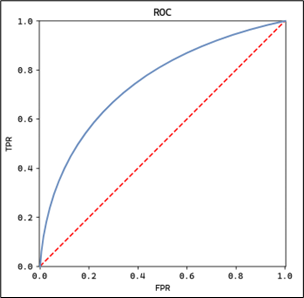
- AUC (Area Under the Curve)
AUC is the area under the ROC curve, which quantifies the overall ability of the model to distinguish between positive and negative classes. A higher AUC indicates better model performance.1
2
3
4
5from sklearn.metrics import roc_auc_score
y_true = [0, 0, 1, 1] # True labels
y_pred = [0, 1, 0, 1] # Predicted labels
print(roc_auc_score(y_true, y_pred))